Setting up Google's Scalable Nearest Neighbors with Docker
Intro to ScaNN and Approximate Nearest Neighbors
For a recent project, I used Google’s ScaNN (Scalable Nearest Neighbors) algorithm. It is an algorithm that came out of Google Research that can be used for many applications, including search and machine learning. In this blog post, I give a bit of motivation for using ScaNN and other Approximate Nearest Neighbors (ANN) methods without going into the math, and then give you the docker configuration and commands you need to get it up and running and try it out yourself.
Nearest Neighbors algorithms are used to search for objects (vectors) that are near to a query object.
Traditional nearest neighbor searches traverse through all potential target objects and calculate the exact distance to find the closest objects. Modern implementations of nearest neighbors use KD Tree and Ball Tree data structures to perform a search, that perform significantly better than brute force nearest neighbors. A KD Tree is a K dimensional tree that partitions the vector space into a tree, reducing the complexity of searching for a vector from O(n) to O(log n). A Ball Tree is also a tree based data structure used for KNN search, but it partitions the data into hyperspheres rather than splitting based on hyperplanes. It can search for data with complexity of O(n log n), but creating the data structure can be time intensive. However, when N becomes millions or billions, even these time complexities can be too slow. ANN methods can bring the runtime complexity to O(1), while sacrificing some result accuracy.
Approximate nearest neighbors algorithms seek to approximate this distance in a performant way to be used in online machine learning or search systems. This can be used for recommendation systems or other applications where exact distance or order is not necessary.
Performance benefits
Approximate nearest neighbors algorithms can take a fraction of the time as exact nearest neighbors. Since they do this by approximating distance, the approximation is part art, and there are many different heuristics and parameters that can be tweaked. Usually there are two or three steps in the algorithm that include building a representation or summary of the targets and the search step. Because of this, there is a lot of ongoing research work on additional improvements to ANN algorithms. There are many different implementations of ANN methods, such as Spotify’s ANNOY (Approximate Nearest Neighbors Oh Yeah), Facebook’s FAISS (Facebook AI Similarity Search), and released this past summer, Google’s ScaNN (Scalable Nearest Neighbors).
 Performance of several leading ANN methods on one dataset. See ANN Benchmarks for a variety of datasets.
This diagram shows performance of several leading ANN methods, with ScaNN performing well on this dataset. There are a lot of considerations to take into account when choosing an ANN algorithm, including speed, recall, distance calculation trade-offs depending on your application, API language availability, and maturity of code.
Approximate Nearest Neighbors and Distance Metrics
In machine learning, it is vital to use the right distance metric to represent the difference between the objects you are representing. Different distance metrics can be used to show the distance between objects in different spaces such as Euclidean space or normed vector spaces.
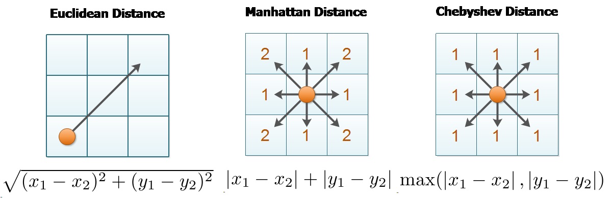 Visualization of differences between Euclidean, Manhattan, and Chebyshev distance. Source
Depending on your task you can prioritize objects based on a metric you define. During my work at MathWorks I worked on the parallel implementation of distance functions, which sped up their computation and also the downstream clustering and machine learning algorithms that used them.
For some applications, exact distance is not as important as finding something nearby. ANN methods are used for solving this type of problem. Google search is a good example of an application like this. Most people don’t care whether the result they are looking for is in position 1 or position 5 in the Google results as long as they can find what they are looking for.
Many times, results after the first page don’t matter at all. Search can be very computationally expensive and it is impossible to search everything on the internet instantaneously, so speed is often preferable to rigidly conforming to an exact distance metric that may not have a direct meaning to users. Because of this, approximate nearest neighbors work focuses on algorithms that prioritize speed with approximate accuracy.
Approximate Nearest Neighbors Heuristics
There are many ways of doing this with heuristics involved at multiple steps. The heuristics include choices made to optimize the representation or indexing of the data and then the distance calculation and querying. Usually the task looks similar to the following: you have one query object (for example: a search phrase) and millions or more potential target objects (document text). One way to approximate this is rather than comparing the query with all targets, a time consuming task, you can calculate a summary object, called a centroid or quantizer, for groups of similar objects. You can limit the search to the nearest quantizers, because some may be distant enough that you don’t want to consider documents near them. Then you can compare the query to only the objects in the close centroids, cutting down the search space. This of course could exclude objects that are closer than the objects you are including at depending on the quantization algorithm to generate the quantizers.
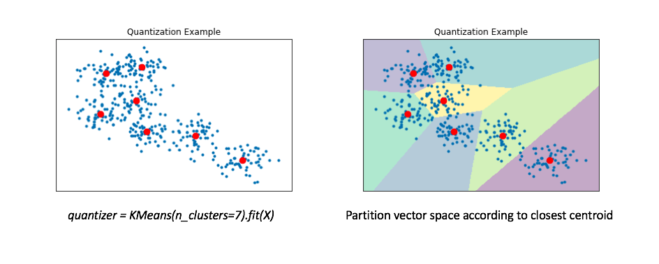 Quantizers and data vectors. Source.
Another performance optimization is to precompute the distance between documents and their centroids and only compare the query document to the centroids directly. Then a combination of the distance between the query and the centroid and the centroid and the target can be used to approximate the total distance. This may or may not be followed by a re-ranking of top candidates to calculate the exact distances, depending on your priority for performance or accuracy.
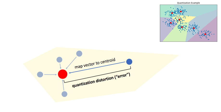 Quantization error is the difference between the centroid and the vector. Source.
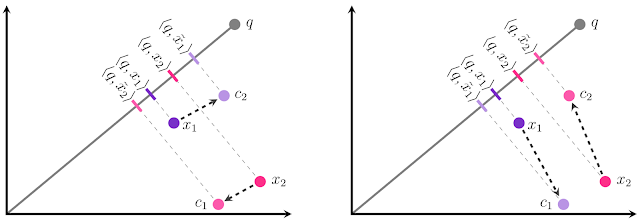
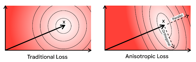
Reconciling the distances between the query and quantizer and between the target and quantizer can be tricky because the directions of the distances can be different, making the distance approximation further off. Orthogonal distances can lead to more error in the approximation.
 Source
Google uses an approach that weights the distances in parallel and orthogonal directions differently to account for this orthogonality.
I will leave the details to the Google blog post and ICML paper and I will demonstrate how to get it up and running with your code.
Trying out ScaNN on Docker
ScaNN was released as a python library. Since ScaNN is research code, they are not releasing binaries for every operating system and distribution. The first release was source and a ubuntu binary, but they since added a manylinux wheel expanding the linux distributions supported which made it easier to run. It is possible to use the library in Linux or MacOS directly, but I prefer to run it in Docker for consistency across operating systems.
To use the steps below you will need to first install docker.
1. Define your Dockerfile
Here is my docker image definition. Save the following in a file name Dockerfile.
FROM ubuntu:18.04

# Install required compiler tools
RUN apt update && apt install -y software-properties-common

# Install python 3.7 and pip
RUN apt update && apt install -y python3.7 python3-pip && apt update

# Install scann
RUN python3.7 -m pip install python-dev-tools
RUN python3.7 -m pip install scann

ADD example.py /
CMD [ "python3.7", "example.py" ]
The example.py used on the last line of the Dockerfile was made from the python code from ScaNN’s example Jupyter script, in order to test it out.
You can download the files in this step here.
2. Build your docker image
With docker installed and running, you can build using the following command:
docker build -t scann_image .
3. Run your docker image
You can run the image you built with the following command:
docker run --rm --name scann scann_image
This will run the image and automatically remove it after executing.
You can mount a local directory on your computer into the docker image using the -v option -v <local dir>:<docker mount path>
docker run --rm --name scann scann_image -v /Users/username/data:/data
4. Incorporate ScaNN into your code
Now that you have ScaNN up and running, you are ready to incorporate the library into your code and experiment. You can start modifying the example code or look at the source code to see how it works.
Use the builder to index the query dataset:
searcher = scann.scann_ops_pybind.builder(normalized_dataset, 10, "dot_product")
              .tree(num_leaves=2000, num_leaves_to_search=100, training_sample_size=250000)
              .score_ah(2, anisotropic_quantization_threshold=0.2).reorder(100).build()
And the searcher to find the nearest neighbors given target vectors:
neighbors, distances = searcher.search_batched(queries)
Have fun using this library!
If you need help with cloud software development,
I offer contracting services.
Email me for more info!